Note
Go to the end to download the full example code.
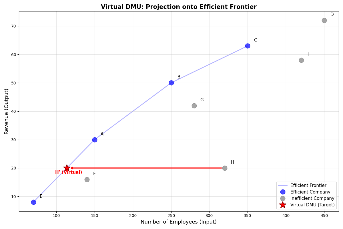
Virtual DMU
This tutorial demonstrates how to compute and visualize virtual DMUs (projections). A virtual DMU represents the target values on the efficient frontier for an inefficient unit.
In Data Envelopment Analysis, when a DMU is identified as inefficient, it is useful to know where it should be on the efficient frontier. This projection is called the “virtual DMU” or “target DMU”, which provides concrete improvement targets for the inefficient unit.
Theory
In an input-oriented VRS model, for an inefficient DMU, the projection onto the efficient frontier is calculated using the efficiency score and slacks:
where:
\(\theta^*\) is the efficiency score (0 < θ* ≤ 1)
\(s^-\) is the input slack (non-negative)
\(s^+\) is the output slack (non-negative)
For an efficient DMU (θ* = 1 and all slacks = 0), the virtual DMU equals the original DMU.
The virtual DMU shows:
How much input can be reduced (through θ* and input slack)
How much output can be increased (through output slack)
The target position on the efficient frontier
Import modules and prepare data
We use real company data with 9 companies, 1 input (Employees), and 1 output (Revenue). This example demonstrates how virtual DMU can be used to set improvement targets for real-world business units.
import matplotlib.pyplot as plt
import pandas as pd
from Pyfrontier.frontier_model import EnvelopDEA

# Create company data
# The data contains: Company name, Number of employees (input), Revenue (output)
# This is real company data showing the relationship between workforce and revenue
data = pd.DataFrame({
    'Company': ['A', 'B', 'C', 'D', 'E', 'F', 'G', 'H', 'I'],
    'Employees': [150, 250, 350, 450, 70, 140, 280, 320, 420],
    'Revenue': [30.0, 50.0, 63.0, 72.0, 8.0, 16.0, 42.0, 20.0, 58.0]
})

print("Company Data:")
print(data)
Company Data:
  Company  Employees  Revenue
0       A        150     30.0
1       B        250     50.0
2       C        350     63.0
3       D        450     72.0
4       E         70      8.0
5       F        140     16.0
6       G        280     42.0
7       H        320     20.0
8       I        420     58.0
Fit VRS input-oriented DEA model
We use Variable Returns to Scale (VRS) with input orientation. This means we want to minimize the number of employees while maintaining the current revenue level.
dea = EnvelopDEA("VRS", "in")
dea.fit(data[['Employees']].values, data[['Revenue']].values)

# Display results for all companies
print("\nDEA Results:")
print("-" * 50)
for i, r in enumerate(dea.result):
    status = "Efficient" if r.is_efficient else "Inefficient"
    print(f"{data.loc[i, 'Company']:8s} Score={r.score:.4f} {status}")
DEA Results:
--------------------------------------------------
A        Score=1.0000 Efficient
B        Score=1.0000 Efficient
C        Score=1.0000 Efficient
D        Score=1.0000 Inefficient
E        Score=1.0000 Efficient
F        Score=0.7078 Inefficient
G        Score=0.7500 Inefficient
H        Score=0.3551 Inefficient
I        Score=0.7418 Inefficient
Visualize efficient frontier and virtual DMU
We plot all companies and show the projection of the most inefficient company (H) onto the efficient frontier using a red arrow.
The arrow shows the direction of improvement from the current position to the target (virtual DMU) on the efficient frontier.
# Separate efficient and inefficient companies
eff_companies = [r for r in dea.result if r.is_efficient]
ineff_companies = [r for r in dea.result if not r.is_efficient]

# Sort efficient companies by input (for frontier line)
eff_sorted = sorted(eff_companies, key=lambda r: r.dmu.input[0])

# Create the plot
plt.figure(figsize=(12, 8))

# Draw efficient frontier line (connecting efficient companies)
plt.plot(
    [d.dmu.input[0] for d in eff_sorted],
    [d.dmu.output[0] for d in eff_sorted],
    '-',
    linewidth=2,
    color='blue',
    alpha=0.3,
    label='Efficient Frontier',
    zorder=1
)

# Plot efficient companies (blue circles)
plt.plot(
    [d.dmu.input[0] for d in eff_companies],
    [d.dmu.output[0] for d in eff_companies],
    'o',
    markersize=12,
    color='blue',
    label='Efficient Company',
    alpha=0.7,
    zorder=3
)

# Plot inefficient companies (gray circles)
plt.plot(
    [d.dmu.input[0] for d in ineff_companies],
    [d.dmu.output[0] for d in ineff_companies],
    'o',
    markersize=12,
    color='gray',
    label='Inefficient Company',
    alpha=0.7,
    zorder=3
)

# Add labels for each company
for i, r in enumerate(dea.result):
    plt.text(
        r.dmu.input[0] + 8,
        r.dmu.output[0] + 1.5,
        data.loc[i, 'Company'],
        fontsize=11,
        ha='left'
    )

# Show projection for the most inefficient company (H, index 7)
target_idx = 7  # H (most inefficient with score ≈ 0.355)
result_h = dea.result[target_idx]
virtual_h = result_h.virtual_dmu
company_name = data.loc[target_idx, 'Company']

# Plot the virtual DMU (target) with a red star
plt.plot(
    virtual_h.input[0],
    virtual_h.output[0],
    '*',
    markersize=18,
    color='red',
    label='Virtual DMU (Target)',
    zorder=5,
    markeredgewidth=1.5,
    markeredgecolor='darkred'
)

# Draw arrow from original to virtual DMU
plt.annotate(
    '',
    xy=(virtual_h.input[0], virtual_h.output[0]),  # Arrow head (target)
    xytext=(result_h.dmu.input[0], result_h.dmu.output[0]),  # Arrow tail (original)
    arrowprops=dict(
        arrowstyle='-|>',
        color='red',
        lw=2.5,
        shrinkA=8,
        shrinkB=8
    )
)

# Add text label for virtual DMU
plt.text(
    virtual_h.input[0] - 15,
    virtual_h.output[0] - 2,
    f"{company_name}' (Virtual)",
    fontsize=11,
    color='red',
    weight='bold'
)

plt.xlabel('Number of Employees (Input)', fontsize=13)
plt.ylabel('Revenue (Output)', fontsize=13)
plt.title('Virtual DMU: Projection onto Efficient Frontier', fontsize=15, weight='bold')
plt.legend(loc='lower right', fontsize=11)
plt.grid(True, alpha=0.3)
plt.tight_layout()
plt.show()
Compare original and virtual DMU values
Let’s examine the numerical values for Company H (the most inefficient company) to understand how the virtual DMU is calculated and what improvements are needed.
print("\n" + "=" * 70)
print(f"Company {company_name}: Original vs Virtual (Target)")
print("=" * 70)

result_h = dea.result[target_idx]  # Company H
original_input = result_h.dmu.input[0]
original_output = result_h.dmu.output[0]
virtual_input = result_h.virtual_dmu.input[0]
virtual_output = result_h.virtual_dmu.output[0]

print(f"Efficiency Score (θ*): {result_h.score:.4f}")
print()
print(f"{'':25s} {'Original':>15s} {'Virtual':>15s} {'Change':>15s}")
print("-" * 70)
print(f"{'Employees (Input)':25s} {original_input:15.1f} {virtual_input:15.4f} "
      f"{virtual_input - original_input:15.4f}")
print(f"{'Revenue (Output)':25s} {original_output:15.1f} {virtual_output:15.4f} "
      f"{virtual_output - original_output:15.4f}")
print()
print("Interpretation:")
print(f"- Employees should be reduced by {original_input - virtual_input:.1f} "
      f"(from {original_input:.0f} to {virtual_input:.1f})")
print(f"- With {virtual_input:.1f} employees, the company can maintain revenue of {virtual_output:.1f}")
print(f"- This represents a {(1 - result_h.score) * 100:.1f}% reduction in workforce needed")
======================================================================
Company H: Original vs Virtual (Target)
======================================================================
Efficiency Score (θ*): 0.3551

                                 Original         Virtual          Change
----------------------------------------------------------------------
Employees (Input)                   320.0        113.6364       -206.3636
Revenue (Output)                     20.0         20.0000          0.0000

Interpretation:
- Employees should be reduced by 206.4 (from 320 to 113.6)
- With 113.6 employees, the company can maintain revenue of 20.0
- This represents a 64.5% reduction in workforce needed
Total running time of the script: (0 minutes 0.192 seconds)